Multimodal models like CLIP have opened up new AI use cases by connecting complex objects like images to text descriptions that are easy to understand, generate, and parse. However, off-the-shelf models like CLIP may not be representative of the data typically seen in specific domains, in which case fine-tuning may be needed to adapt the model to that domain.

This post shows how to fine-tune the CLIP model on cartoon images from The New Yorker Magazine and joke captions for those cartoons. It is based on https://www.capcon.dev/, a dataset for various tasks associated with The New Yorker’s cartoon contest. One of the tasks is to take a cartoon image and predict the appropriate caption from a list of possible captions. Let’s see how we can fine-tune CLIP for this task.

Data

The data is hosted and publicly available at gs://datachain-demo/newyorker_caption_contest, and it has two parts:

• images: A folder of JPEG files, each representing a cartoon image.
• new_yorker_meta.parquet: A parquet file with metadata about the images, including multiple choices of captions for the image and the correct caption choice.

To work with this data, we will use the open-source library datachain, which helps to wrangle unstructured data like this into a more structured format (disclaimer: I helped develop datachain). All of the code used in this post is available in a Jupyter Notebook in GitHub, or you can run it in Colab.

To start, we read both the images and metadata from their sources and then join them according to filename (which is available as a column in the metadata):

from datachain import C, DataChain
from datachain.sql.functions import path

img_dc = DataChain.from_storage("gs://datachain-demo/newyorker_caption_contest/images", type="image", anon=True)
meta_dc = DataChain.from_parquet("gs://datachain-demo/newyorker_caption_contest/new_yorker_meta.parquet")
dc = img_dc.mutate(filename=path.name(C("file.path"))).merge(meta_dc, on="filename")

The code first creates a dataset img_dc from images in a directory, storing the essential information about each file, which we will use later to read the images. Then, it creates a dataset meta_dc from the parquet file of metadata. Finally, it merges these two based on the image filename. img_dc contains a column file.path with the full path to the file, and img_dc.mutate(filename=path.name(C("file.path"))) extracts only the last part of that path, which matches the contents of the filename column in meta_dc. The merged dc dataset has both the file info and metadata for each image.

We can view a sample of the data by filtering and collecting the data like this:

sample = dc.filter(C("file.path").endswith("/371.jpeg")).limit(1)
sample_results = list(sample.collect("file", "caption_choices", "label"))

This limits the data to the image ending in /371.jpeg and collects only the columns "file", "caption_choices", "label". The resulting output includes an ImageFile (see below), a list of possible captions, and a label for the letter choice of the correct caption. You may end up with slightly different results since there are multiple rows per image with different caption choices.

[(ImageFile(source='gs://datachain-demo', path='newyorker_caption_contest/images/371.jpeg', size=25555, version='1719848719616822', etag='CLaWgOCXhocDEAE=', is_latest=True, last_modified=datetime.datetime(2024, 7, 1, 15, 45, 19, 669000, tzinfo=datetime.timezone.utc), location=None, vtype=''),
  ["I feel like we've gotten a little soft, Lex.",
   "Hold on, the Senate Committee on Women's Health is getting out.",
   "I know a specialist, but he's in prison.",
   'Six rounds. Nine lives. You do the math.',
   'Growth has exceeded our projections.'],
  'D')]

We can get the image itself from the ImageFile object using its read() method:

example = sample_results[0]
example[0].read()

Image from https://www.capcon.dev/ via The New Yorker

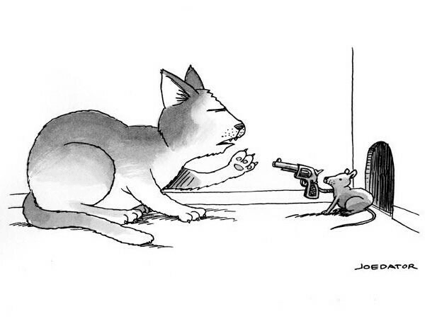
In this sample, we have a cartoon of a mouse pointing a gun at the cat, with the correct caption being option D, which reads, “Six rounds. Nine lives. You do the math.”

Applying a base CLIP model

We can apply CLIP to this data to predict the likelihood of each caption. This is similar to the base architecture of CLIP, which uses contrastive learning to take an image and discern the most likely caption from a batch of text captions (and vice versa). During training, CLIP gets batches of image-text pairs as input, with each image mapped to its text caption. For each batch, CLIP calculates the cosine similarity of each image to each text in the batch, so that it has not only the similarities of the matches but also of every mismatched image-text pair (see the image below). It then treats this as a classification problem where the match is considered the correct label and the mismatches are considered the incorrect labels. During inference, this can be used as a zero-shot predictor by feeding in an image and batch of captions, for which CLIP will return the probability of each caption. For a deeper dive into CLIP, see the original OpenAI post about it, or Chip Huyen has a nice summary of how it works here.

Image from https://openai.com/index/clip/ Image from https://openai.com/index/clip/

For the cartoon dataset, we can feed in our sample image and the caption choices to get back the probability that each is a correct match. Here’s how that looks in code:

import clip
import torch

device = "cuda" if torch.cuda.is_available() else "cpu"
model, preprocess = clip.load("ViT-B/32", device=device)

image = example[0].read()
image = preprocess(image).unsqueeze(0).to(device)
text = clip.tokenize(example[1]).to(device)
logits_per_image, logits_per_text = model(image, text)
logits_per_image.softmax(dim=1)[0]

First, we load the ViT-B/32 pre-trained model and image preprocessor onto the device. Then, we transform the image into the expected tensor input and tokenize the text captions to do the same. Next, we run the model on those transformed inputs to get the logit similarity scores of the image to each text, and finally run a softmax function to get a relative probability for each text caption.

The output shows that CLIP can already confidently predict the correct caption for this example, since caption D (the fourth caption) has a probability of 0.9844 (if you try this yourself, you may have different caption choices in your example, which may lead to different results):

tensor([0.0047, 0.0013, 0.0029, 0.9844, 0.0067], grad_fn=<SelectBackward0>)

Creating a training dataset

Now that we know how to apply CLIP to predict captions, we can build a training dataset for fine-tuning the model. Let’s get the similarity scores for a random 10 images (you can increase to a larger size but we will keep it small here to make it easy to quickly follow along on a laptop CPU). Here’s the code to do that:

from datachain.torch import clip_similarity_scores

train_dc = dc.shuffle().limit(10).save("newyorker_caption_contest_train")
train_dc = train_dc.map(
    func=lambda img_file, txt: clip_similarity_scores(img_file.read(), txt, model, preprocess, clip.tokenize, prob=True)[0],
    params=["file", "caption_choices"],
    output={"scores": list[float]}
)

First, we shuffle and save 10 images from the dataset. Then, we use the map() method to to apply a function to each record and save the result as a new column. We use the utility function clip_similarity_scores, which performs the steps from the previous section in one line to get the caption probabilities. The input to the map() function is defined by params=["file", "caption_choices"], and the output column is defined by output={"scores": list[float]}.

For training, we also need the ground truth of the correct captions, so we again use map() to calculate the index of the correct caption for each record, along with the CLIP probability of that caption so we can see how well baseline CLIP is performing:

import string

def label_ind(label):
    return string.ascii_uppercase.index(label)

def label_prob(scores, label_ind):
    return scores[label_ind]

train_dc = (
    train_dc.map(label_ind, params=["label"], output={"label_ind": int})
    .map(label_prob, params=["scores", "label_ind"], output={"label_prob": float})
)
train_dc = train_dc.save()

We can run train_dc.avg("label_prob") to get the average probability of the correct caption for the training sample. The average will depend on the random samples in your training dataset, but you should see a much lower value than the sample image above, so it seems the other images are not so easy for baseline CLIP to correctly predict.

Fine-tuning

To fine-tune CLIP, we need to create a train() function to loop over the training data and update the model:

def train(loader, model, optimizer, epochs=5):
    if device == "cuda":
        model = model.float()
    loss_func = torch.nn.CrossEntropyLoss()

    for epoch in range(epochs):
        total_loss = 0
        for images, texts, labels in loader:
            optimizer.zero_grad()
            batch_loss = 0
            for image, text, label in zip(images, texts, labels):
                image = image.to(device).unsqueeze(0)
                text = text.to(device)
                label = label.to(device).unsqueeze(0)

                logits_per_image, logits_per_text = model(image, text)

                batch_loss += loss_func(logits_per_image, label)
            batch_loss.backward()
            optimizer.step()
            batch_loss = batch_loss.item()
            total_loss += batch_loss
        print(f"loss for epoch {epoch}: {total_loss}")

For each pairing of image to text captions, the function calculates the logit similarity scores, uses the correct label index to apply the loss function, and performs a backward pass to update the model.

This is very similar to how base CLIP works, except for one difference. Base CLIP expects each batch to contain image-text pairs, where each image has a single corresponding text, and CLIP must get incorrect texts from the other samples in the batch for contrastive learning (see the image above). With the cartoon dataset, each image already has not only the corresponding correct text caption, but also multiple incorrect text captions. Therefore, instead of relying on the other samples in the batch for contrastive learning, the function above relies only on the text captions choices provided for that image.

To feed the training data into this function, we need to generate a PyTorch dataset and data loader and pass the loader to the train() function along with an optimizer:

from torch.utils.data import DataLoader

ds = train_dc.select("file", "caption_choices", "label_ind").to_pytorch(
    transform=preprocess,
    tokenizer=clip.tokenize,
)

loader = DataLoader(ds, batch_size=2)
optimizer = torch.optim.Adam(model.parameters(), lr=1e-4)
train(loader, model, optimizer)

The code above selects the columns needed for training ("file", "caption_choices", "label_ind"), and then calls to_pytorch() with the CLIP preprocessor and tokenizer, which returns a PyTorch IterableDataset with the preprocessed image tensors, tokenized text, and label indices. Next, the code creates a PyTorch DataLoader and optimizer and passes them to train() to start training.

Since we are using a tiny dataset, we can quickly see the model fit to the sample and the loss decreases dramatically:

loss for epoch 0: 5.243085099384018
loss for epoch 1: 6.937912189641793e-05
loss for epoch 2: 0.0006402461804100312
loss for epoch 3: 0.0009484810252615716
loss for epoch 4: 0.00019728825191123178

This should set off alarm bells about overfitting, but for this exercise, it’s useful to see that train() is doing what we expect: learning the correct captions from the training dataset. We can confirm by calculating the predicted probability of the correct caption for each image in the training data using the fine-tuned model:

train_dc = train_dc.map(
    func=lambda img_file, txt: clip_similarity_scores(img_file.read(), txt, model, preprocess, clip.tokenize, prob=True)[0],
    params=["file", "caption_choices"],
    output={"scores_fine_tune": list[float]}
)

train_dc = train_dc.map(label_prob, params=["scores_fine_tune", "label_ind"], output={"label_prob_fine_tune": float})

The above code is the same that was used above to calculate the probability before fine-tuning. Running train_dc.avg("label_prob_fine_tune") outputs an average predicted probability >0.99, so it looks like the fine-tuning worked as expected.

This is an artificial example but hopefully gives you an idea of how to fine-tune CLIP. To solve the task of predicting the correct caption in a more robust way, you would want to take a much larger sample and evaluate against a held-out sample of images and texts that hadn’t been seen during training. When trying that, you may find that CLIP does not perform so well at generalizing to the caption prediction problem, which should not be too surprising since CLIP was built to understand the contents of images rather than understanding jokes. CLIP relies on a relatively simple text encoder, and it may be worth exploring different text encoders for that task. This goes beyond fine tuning and this post, but now that you know how to train CLIP, you can try out this idea or bring your own ideas for how to adapt CLIP to your multimodal use cases.