From Jupyter Notebook to DVC pipeline for reproducible ML experiments

While every data scientist has their own methods and approaches to conducting data science, there is one tool that nearly everyone in the field uses: Jupyter Notebook. Its ease of use makes it the perfect tool for prototyping, usually resulting in a script in which we preprocess the data, do a train/test split, train our model, and evaluate it.

However, once we have a decent prototype, the subsequent iterations generally don’t touch most of the code. Instead, we tend to focus on tweaking feature engineering parameters and tuning model hyperparameters. At this point, we really start experimenting, trying to answer questions such as “What happens if I increase the learning rate?” and “What’s the optimal batch size?”

It will take numerous experiments to get to an acceptable level of performance for our model. But with so many experiments, it becomes difficult to keep track of the changes. In turn, this makes it difficult to go back in time to a certain point and see what combination of data, code, and parameters constituted a specific experiment. In other words, we cannot reproduce our experiments.

We can solve our need for reproducibility by transforming our notebook into a codified pipeline with defined inputs and outputs. This will allow us to then save every experiment that modifies the inputs, pipeline, or outputs. In this guide, we will explore how to do this using DVC. It extends Git so that in addition to code and parameters we can track and version data and models.

What we’ll be doing

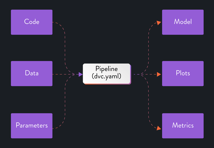
While a pipeline typically consists of multiple stages, transforming our notebook straight into a multi-stage DVC pipeline may seem somewhat daunting. For the sake of simplicity, we will create a pipeline with just one stage for now: run all of the code in our notebook. Just like any other pipeline, we will have defined inputs (data and parameters) and outputs (model, evaluation metrics, and plots).

To achieve this, we will wrap our notebook with Papermill. With this tool, we can parameterize our notebook and run experiments from our CLI with a single command.

Throughout this guide, we will do the following:

1. Parameterize a notebook using Papermill;
2. Create a single-stage pipeline with DVC;
3. Version our data, model, and other large artifacts using DVC; and
4. Run multiple experiments using the new pipeline.

As an example project, we will be using a notebook I created that trains a classifier for Pokémon sprites. You can find this project in the repository here. Make sure to follow the instructions in README.md to set up the development environment and to git checkout snapshot-jupyter to get our starting point for this guide.

Of course, you can also follow along using a notebook you created yourself! In that case, you will at least need to install dvc and papermill. You will also need to initialize DVC through dvc init.

Guide

Stages in a DVC pipeline consist of commands as we could run them in our own terminal. As such, we need a way to run the contents of our notebook from our command line. This is where Papermill comes in. With the following command we execute the entire notebook as a single unit without changing its contents:

$ papermill \
notebooks/pokemon_classifier.ipynb \
outputs/completed_notebook.ipynb

The result is saved as a new notebook in outputs/completed_notebook.ipynb.

Parameterize notebook

While we would technically have a DVC pipeline if we added this command as a stage, its usefulness would be somewhat limited. After all, the result would be the same every time we execute the command. To start experimenting with our pipeline, we need to parameterize our notebook. We do so by creating a single cell at the top of our notebook where we declare the parameters:

SEED: int = 42
POKEMON_TYPE_TRAIN: str = "Water"

SOURCE_DIRECTORY: str = "data/external"
DESTINATION_DIRECTORY: str = "data/processed"
TRAIN_DATA_IMAGES: str = "images-gen-1-8"
TRAIN_DATA_LABELS: str = "stats/pokemon-gen-1-8.csv"

MODEL_TEST_SIZE: float = 0.2
MODEL_LEARNING_RATE: float = 0.001
MODEL_EPOCHS: int = 10
MODEL_BATCH_SIZE: int = 120

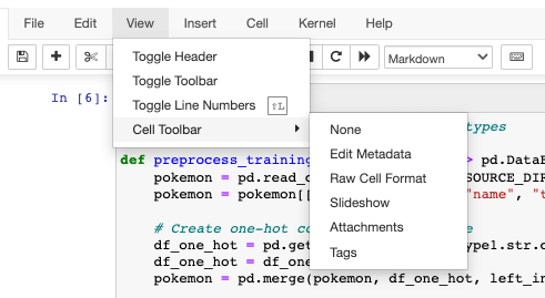
Papermill needs a parameters tag to recognize this cell as the one containing our parameters. To add this tag to the cell, we go to View / Cell Toolbar and enable Tags. Afterward, we type in parameters in the top right corner of our cell.

Enabling Tags for Jupyter Notebook cells

We can now replace hard-coded parameters in our notebook with references to the variables we defined. For example, we change the following section of code like so:

estimator = model.fit(X_train, y_train,
                      validation_data = (X_test, y_test),
                      class_weight = calculate_class_weights(y_train),
-                     epochs = 10,
+                     epochs = MODEL_EPOCHS,
-                     batch_size = 120,
+                     batch_size = MODEL_BATCH_SIZE,
                      verbose = 1)

Now we can run our notebook through Papermill with changed parameters:

$ papermill \
notebooks/pokemon_classifier.ipynb \
outputs/completed_notebook.ipynb \
-p MODEL_EPOCHS 15 \
-p MODEL_BATCH_SIZE 160

Create DVC pipeline

With our parameterized notebook in place, we can create our pipeline with DVC. Our pipeline consists of stages (in this case: one stage) and has inputs and outputs. For our model, the inputs will be the required datasets and our notebook. The pipeline’s outputs will be the model itself, a graph showing the training process, and a confusion matrix for the model’s predictions.

Additionally, a pipeline can have metrics and plots. We will define several metrics that allow us to compare model performance across different experiments, such as accuracy and F1 scores.

Our inputs, pipeline, and outputs

A DVC pipeline is defined in a dedicated dvc.yaml file. We can add stages manually in this file, which you generally want to do when building complex, multi-stage pipelines. However, to get started, it’s probably easier if we use the dvc stage add command. We use the -n option to provide a name for the stage, the -d option to specify our dependencies, the -o option to specify our outputs, and the -M option to specify our metrics file. Lastly, we type in the command that DVC should execute for that stage:

$ dvc stage add \
-n run_notebook \
-d notebooks/pokemon_classifier.ipynb \
-d data/external/images-gen-1-8 \
-d data/external/stats/pokemon-gen-1-8.csv \
-o data/processed/pokemon \
-o data/processed/pokemon.csv \
-o data/processed/pokemon-with-image-paths.csv \
-o outputs/model.pckl \
-o outputs/confusion_matrix.png \
-o outputs/train_history.png \
-M outputs/metrics.yaml \
papermill notebooks/pokemon_classifier.ipynb outputs/pokemon_classifier_out.ipynb

The uppercase -M option (as opposed to the lowercase -m option) tells DVC not to track the resulting metrics file. We typically want to do this with metrics because the files are small enough to be tracked by Git directly.

The resulting dvc.yaml looks as follows:

stages:
  run_notebook:
    cmd: >
      papermill notebooks/pokemon_classifier.ipynb
      outputs/pokemon_classifier_out.ipynb
    deps:
      - notebooks/pokemon_classifier.ipynb
      - data/external/images-gen-1-8
      - data/external/stats/pokemon-gen-1-8.csv
    outs:
      - data/processed/pokemon
      - data/processed/pokemon.csv
      - data/processed/pokemon-with-image-paths.csv
      - outputs/model.pckl
      - outputs/confusion_matrix.png
      - outputs/train_history.png
    metrics:
      - outputs/metrics.yaml:
          cache: false

With that, we have our pipeline in its basic form! We can run the pipeline with the dvc repro command, and DVC will execute our notebook. We have yet to specify our parameters, however. Otherwise, every pipeline run would utilize the default parameters we defined in our notebook.

DVC parses in the values for parameters from another YAML file: params.yaml. We can declare the same parameters here that we previously incorporated in our notebook. To provide a little bit of structure, let’s also group them in sections:

base:
  seed: 42
  pokemon_type_train: 'Water'

data_preprocess:
  source_directory: 'data/external'
  destination_directory: 'data/processed'
  dataset_labels: 'stats/pokemon-gen-1-8.csv'
  dataset_images: 'images-gen-1-8'

train:
  test_size: 0.2
  learning_rate: 0.001
  epochs: 15
  batch_size: 120

We can now update our pipeline in dvc.yaml to read the parameters from params.yaml. The file is detected automatically by DVC and we can parse the values into the papermill command with the -p option. The result will look like this:

stages:
  run_notebook:
    cmd: >
      papermill
      notebooks/pokemon_classifier.ipynb
      outputs/pokemon_classifier_out.ipynb
+     -p SEED ${base.seed}
+     -p POKEMON_TYPE_TRAIN ${base.pokemon_type_train}
+     -p SOURCE_DIRECTORY ${data_preprocess.source_directory}
+     -p DESTINATION_DIRECTORY ${data_preprocess.destination_directory}
+     -p TRAIN_DATA_IMAGES ${data_preprocess.dataset_images}
+     -p TRAIN_DATA_LABELS ${data_preprocess.dataset_labels}
+     -p MODEL_TEST_SIZE ${train.test_size}
+     -p MODEL_LEARNING_RATE ${train.learning_rate}
+     -p MODEL_EPOCHS ${train.epochs}
+     -p MODEL_BATCH_SIZE ${train.batch_size}
    deps:
    - notebooks/pokemon_classifier.ipynb
    - data/external/images-gen-1-8
    - data/external/stats/pokemon-gen-1-8.csv
    outs:
    - data/processed/pokemon
    - data/processed/pokemon.csv
    - data/processed/pokemon-with-image-paths.csv
    - outputs/model.pckl
    - outputs/confusion_matrix.png
    - outputs/train_history.png
    metrics:
    - outputs/metrics.yaml:
        cache: false

And with that, we have our pipeline ready for use! Before we start running experiments with it, however, let’s ensure everything is tracked and versioned properly so we can reproduce our experiments later on.

Version our data, models, and plots with DVC

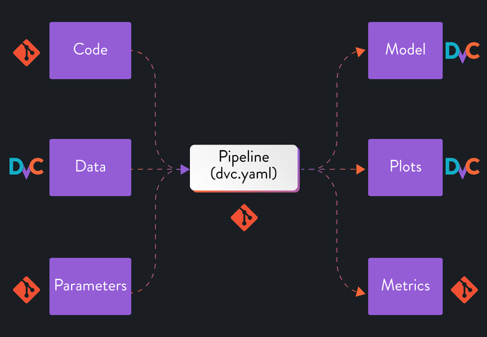
As we discussed earlier, we want to version every component of our experiments to achieve true reproducibility: code, parameters, data, models, metrics, and plots. We want to version small files (usually text) with Git and larger files with DVC. That principle gives us the following split between the two:

Every component of our experiment is versioned either by Git or DVC

When we created our pipeline in the previous step, DVC automatically started tracking the outputs we defined and listed them in our .gitignore. On the other hand, the metrics file is ignored by DVC and still tracked by Git (cache: false), because we added it with the upper case -M option. If we wanted to track the metrics with DVC as well, we could change this in our dvc.yaml.

There is one last output of the pipeline we haven't yet accounted for: outputs/completed_notebook.ipynb. Because it's a rather large file that we don't really need for anything, we can simply add it to our .gitignore. After all, we can always reproduce it by rerunning our pipeline!

With that, every component (of importance) in our project is now versioned by Git or DVC. That means we now have the reproducible pipeline we set out to create: we can go back to any experiment and get the precise combination of code, data, parameters, and results. This will make it much easier to conduct experiments, find the best-performing model, and collaborate with teammates.

Let’s take our pipeline for a ride and run some experiments!

Running experiments

There are two ways in which we can run experiments with our newly defined pipeline. The first one utilizes our good ol’ command line interface. We can use dvc exp run to run an experiment after we have changed the parameters in params.yaml, or we could change the parameters in the command itself with the -S option. The following command would trigger a new experiment with an updated number of epochs, for example:

$ dvc exp run -S 'train.epochs=25'

However, if we’re using Visual Studio Code as our IDE of choice, we can also use the DVC extension to run and visualize experiments through a graphical user interface. We can go to the experiment table and, from there, modify, queue, and run new experiments. The results will be shown below each other, providing an easy way to compare their outcomes.

Now, all there’s left to do is to start experimenting and find the best possible model! Once we have drawn our conclusions from experimenting, we can pick the best-performing experiment and start using the model it put forth.

Conclusions

Throughout this guide, we transformed a Jupyter Notebook into a codified pipeline for reproducible experiments. We used Papermill to parameterize our notebook so that we could run it with a single command and then created a pipeline in DVC to run that command for us.

With our DVC pipeline tracking and versioning every experiment, we can discover which combination of code, data, and parameters provides the best results. Comparing experiments is especially easy when using the experiment table in the DVC extension for Visual Studio Code.

From this point onwards, we can still make a few improvements to our pipeline. For one, we could leverage DVC to generate our plots rather than render them as images from our notebook. This would allow us to compare experiments visually in a similar manner to how DVC can visualize an experiments table. To learn more about this, please refer to the docs.

Another improvement would be to break up our single-stage pipeline into different stages with coherent units of code (e.g., preprocess, train, and evaluate). Our current implementation runs the entire notebook for every single experiment, even though the data preprocessing doesn’t change between experiments. With a multi-stage pipeline, DVC could track changes to the in- and outputs for every stage and automatically determine which stages it can skip because nothing has changed. This saves time and resources, especially in computationally heavy projects.

$ dvc dag
+-------------------+
| data/external.dvc |
+-------------------+
          *
          *
          *
 +-----------------+
 | data_preprocess |
 +-----------------+
          *
          *
          *
    +-----------+
    | data_load |
    +-----------+
          *
          *
          *
      +-------+
      | train |
      +-------+
          *
          *
          *
    +----------+
    | evaluate |
    +----------+

If you want to learn how to transform a notebook into a multi-stage pipeline, I recommend taking a look at our course: Iterative tools for Data Scientists and Analysts. It is completely free to follow, and module 3 covers this process in depth.

We might also write a future guide about this, so let us know if you would be interested in seeing this content. Make sure to join our Discord server if you have any questions or want to discuss this post further!